

- By Hans D. Baumann, PhD, PE
- Automation Basics
Summary
By Hans D. Baumann, PhD, PE
Understanding and reducing noise from control valves is an important consideration for process facilities, especially those close to residential areas. After years of working with this issue, the author developed a simple, graphical method to estimate water noise.
The underlying algorithms were found based on fundamental laws of fluid mechanics and acoustics, which enable the calculation of the sound levels of turbulent or cavitating water, and thereby simplify the International Electrotechnical Commission (IEC) standard method, while at the same time improving accuracy. A simplified graphical method can be a handier alternative to a computerized method. Although this method, as exhibited, is valid only for water, it could be modified for other fluids as long as the specific gravity and sonic velocity are accounted for.
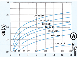
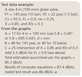
The results are three graphs (A, B, and C), which condense the equations of the underlying mathematics. The first graph, A, shows sound levels as a function of the given downstream pipe diameter either in inches or in millimeters and as a function of the relative flow capacity (Cv/D2). (D is in inches, or 0.0016 x d2 if d is given in mm). The graph also incorporates the pipe's transmission loss based on schedule 40 pipe (for schedule 80, see below.)
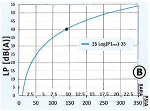
The next step is to consult graph B based on the absolute inlet pressure to the valve either in psia or bar absolute. Add the dB(A) numbers found to the numbers given in graph A and proceed to graph C.
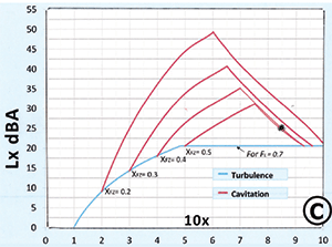
Go to graph C. Before you can read the numbers, find the valve's pressure ratio, where X = (P1 - P2 / P1 - Pv), or 0.03 bar absolute at 70°F). This graph incorporates both the turbulence (blue) as well as the cavitation (red) sound level components of water. First, consult your valve's catalog information to find the Xfz (incipient cavitation) factor for the chosen valve and valve travel. If unknown, check the table below for an approximate value. Take your pressure ratio factor X (see above) and multiply it by 10. Now go to the bottom of graph C. If X is smaller than Xfz, then go to the blue line and read the corresponding dB(A) values on the left. If X is larger than Xfz, go to the red lines (indicating you have cavitation) and read the dB(A) numbers corresponding to the red line based on your given Xfz number and intersecting with the 10X line.
Now add all dB(A) numbers from A, B, and C, and you will have the estimated sound level 1 meter from the pipe wall. This method is based on the mathematical equations shown in the resources and is considered accurate to within ±5 dB(A).
Here are some modifiers to note, if applicable:
If your pipe is schedule 80, add 4 dB. In case this is a rotary valve, add 3 dB to the total.
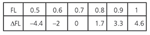
If your FL factor is different from 0.7, then add the following ∆FL numbers:
In cases where your fluid is something other than water, add the following factor
NL = 20log (1448/Ci fluid) + 15log (Þfluid / 998)\, where Cifluid = fluid speed of sound (ft/sec)
and þfluid = density of fluid (lbs/ft3).
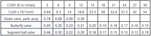
Tabulation of Xfz factors
|
||
|
|
|
|
Reader Feedback
We want to hear from you! Please send us your comments and questions about this topic to InTechmagazine@isa.org.