Data filtering in process automation systems

• By Brian M. Hrankowsky, Joseph S. Alford, PhD, R. Russell Rhinehart
• InTech

Summary

Removing unwanted data signal components or features

By Joseph. S. Alford, PhD, Brian M. Hrankowsky, and R. Russell Rhinehart

A data filter is a device, algorithm, or process that removes some unwanted components or features from a data signal. The unwanted component may be random noise (perhaps from mixing turbulence or mechanical vibrations), spurious outlier events (such as missed data packets or isolated spikes), or a periodic confusion (for instance from power or rotational harmonics).

The data signal may be a direct measurement or a virtual estimate of either a measurement or a key performance metric, which are inputs to process automation (control, historian) or enterprise management systems. In many cases, some preprocessing (data filtering) is desired before the input is presented to a controller or used in a trend plot for process representation.

Smoothing data and eliminating outliers have several advantages. For example, reducing noise in the derivative portion of a controller could lead to greater use of the derivative term in proportional, integral, derivative (PID) control (and, therefore, improved control). Data filtering also reduces distracting features in trend plots. And, less noise in a control loop's controlled variable can contribute to reduced variation in the controller output. However, data filtering can also have negative consequences, such as hiding real problems occurring or developing in a process or its equipment. It can also present a skewed (i.e., invalid) view of the magnitude and duration of real spikes occurring in the process. And, in general, data filtering causes a delay or a lag that can interfere with control. The engineer must understand that the real process value and the measured or displayed value are not the same thing.

In some applications, little or no data filtering is recommended. This is often the case with signals sent to alarm algorithms or to data collection systems, and those presented on a human-machine interface for critical process parameters (i.e., those impacting product quality) in "current Good Manufacturing Practice" (cGMP) regulated processes. In such applications, it is important to monitor and record true details of process excursions, not to reduce the perceived magnitude or extend the perceived duration of process spikes through filtering.

In some cases, there may be value in using and recording two forms of a process variable, one being the raw data from an instrument (useful in analyzing the details of a process or system excursion) and the second a filtered version useful for PID control or trend plots for presentation and publication.

Several different data filtering technologies are utilized in industrial automation systems. This article discusses some of them, including comments on pros and cons, and organizes them in categories of noise removal, outlier removal, and stray signal removal.

Most control systems (distributed control systems, programmable logic controllers, or PCs) do not have a broad menu of data filtering options to choose from; some have only one or two that are commonly applied in the process industry. However, most systems have some form of calculation blocks available for users to program or configure as part of application software, so users can implement whatever data filtering algorithm is deemed appropriate.

Noise removal methods

The concept is that the process is holding a steady value in time and that the signal is corrupted by random fluctuations. The objective of the filter is to reveal the underlying value.

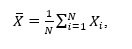
Moving average filter (MA): A moving average filter reports the conventional average of data in a window:

 
in which i = 1 indicates the most recent data, and the average is over the past N data values.

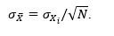
This is termed a window of the data. At each sampling, the window moves, the newest data enters, and the oldest leaves. The user needs to specify the window length either as a time duration or as the number of the data in the window. The more data, the lower the variability is on average. At a steady condition (the nominal value is not changing, but the measurements fluctuate randomly due to noise effects), the variability of the average is related to the variability of the individual data:

 

The √N impact is true for any measure of variability, such as range. Note: Variation cannot be eliminated by averaging, just attenuated. The user needs to choose the value of N. A larger N means less variation, but it also means that it will take longer for the average to move to the proximity of the new value when the data value changes.

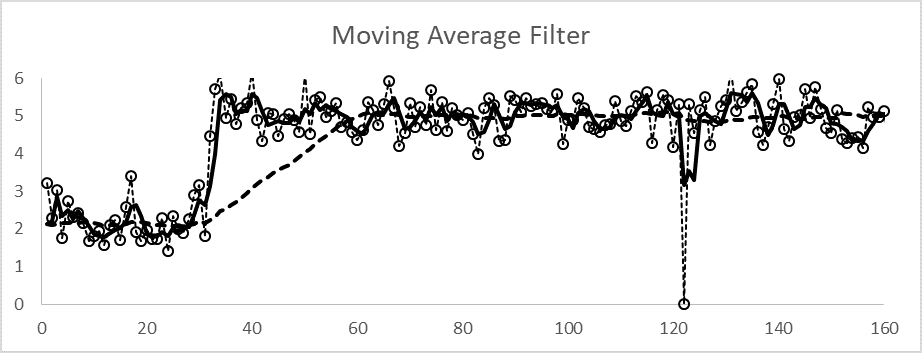
Figure 1 reveals a process (data are the markers) that is initially at a noisy steady state at a nominal value of 2, then makes a step change to a new value of 5 at the 30^th sampling. The data value is on the vertical axis, and the sample number is on the horizontal axis. A data spike, a spurious signal with a value of zero, occurs at sampling 120. The thin dashed line connects the data dots to help reveal the trend. Subsequent figures will show results of diverse filtering methods on the same data.

In figure 1, the solid line represents the moving average filter with N=3 and the dashed line with N=30. Note several features:

• The MA with N=3 makes a more rapid rise to the new data value, but its variation is larger than the MA with N=30.
• The character of an MA filter response to a step change in the signal is a linear ramp toward the new value, which lasts N samples.
• The response to the one-time outlier is a pulse that has a duration of N samples and a magnitude of 1/N^th of the outlier deviation.

---

An advantage of the MA filter is that the concept of averaging is commonly understood, and the tuning choice of window length N is easily related. For example, moving averages are common in reporting the performance of a company stock. When periodic disturbances are present, a window length chosen to match the period will result in a signal that moves to the new average in one period. However, the algorithm causes some delay in process alarms and process control applications realizing and responding to a sudden process change. The algorithm does not reject data outliers.

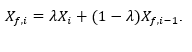
First-order filter (FoF): A first-order filter has several alternate names, including exponentially weighted moving average (EWMA) and autoregressive moving average (ARMA). A FoF represents the analog device methods for filtering an electronic resistor-capacitor or pneumatic restriction and bellows, but it can be digitally performed. The advantage is that it is computationally simpler than an MA filter, which must store and process all of the data in the window. The FoF equation is:

Here lambda, λ, is the filter factor (it is not related to lambda tuning). It ranges between 0 and 1, 0 < λ < 1.

X_i is the most recent data measurement; Xf\,i_-1 is the prior filtered value; and X_f\,i is the new filtered value. If one derives the equation as an approximation to the moving average method, essentially:

λ=¹⁄_N.

Some vendors use the symbol f for the filter factor, and some switch the the λ and (1-λ) weighting. If one derives the FoF from the differential equation representing a first-order RC circuit, then:

λ=1-e^-Δt/τ ,

where Δt is the sampling interval, and τ is the time constant. With substantial filtering, the time constant is approximately related to the number of data, τ≅ΔtN. The user needs to be aware of the manner in which the vendor presents the filter.

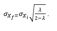
The FoF also tempers, but does not remove, noise. Here, if the process is steady, with random fluctuations, the relation for variability attenuation is:

The user chooses the value of λ (or alternately ƒ for τ) to temper the noise. Although the benefit of a FoF over the MA filter is computational simplicity, the negative is the persisting influence of long past data. In the MA, once a data value is out of the window, it no longer influences the average. However, in a FoF the past values are exponentially weighted, fading in time, but never totally leaving.

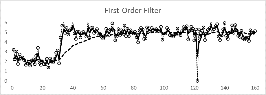
Figure 2 illustrates the performance of a FoF. The filtered value makes a first-order response to a change in the process. The lambda values of (solid line) and (dashed line) are chosen to represent the same noise reduction obtained with the N=3 and N=30 values of the MA filter, λ=2⁄(N+1).

Note:

• Both filtered values show an exponential rise to the new value, requiring three-to-four time constants, a period of N≅3.5/λ, to make about 97 percent of the change to reach the proximity of the new value.
• After the spike at sample 120, there is a progressive relaxation back to the filtered value.

---

The key advantage of the FoF over the MA filter is that the algorithm is computationally simple. However, the interpretation of the filter factor or time constant is less intuitive than choosing N in a moving average. And, the FoF does not reject outliers.

In either the MA or FoF the user must choose the filter coefficient value to best balance the lag or ramp period and to desirably temper the variation. In either case, the user needs to realize that the lag can be detrimental to control if it is similar in magnitude to the primary time constant or dead time of the process. The filter time constant should not be selected to be any greater than 1/5 the primary time constant. Filtering might be in any number of places (e.g., on the instrument or sensor, in the data acquisition transmittal system, on the I/O cards, in the control device, or as an option in the control algorithm). With a correctly implemented controller utilizing derivative, mode, filtering of the CV may not be necessary at all. Both algorithms hide the true magnitude and duration of process spikes.

Butterworth filter: Butterworth filters are a family of filters for addressing low, high, or band-limited frequency noise. The first-order low-pass Butterworth filter is the same as a FoF. As the order of the filter increases, the sharper the magnitude response is at the cutoff frequency, but more lag is introduced into the system. The FoF removes high-frequency noise (data-to-data variation) but tracks the average. However, in some frequency-based electronic applications, the user desires to have both a low-pass and high-pass filter. Although popular in electronic applications, it is rarely relevant in process monitoring or control. Some control systems use a second-order low-pass Butterworth filter due to its truer response to process changes (i.e., a lower cutoff frequency can be used to get the same desired attenuation).

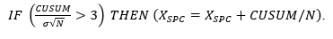
Statistical filter: One of several approaches is based on a Six Sigma (statistical process control) desire to prevent tampering. In the filters discussed, even at steady conditions, the filter will continually report small deviations, and if used in automatic control, the controller will seek to correct this residual noise. The prevent-tampering concept is to hold a single filtered value until there is statistically confident evidence that the process value has changed, then change the filtered value. In one technique, a cumulative sum (CUSUM) of deviations of measurement from the filtered value is the observed metric. If the CUSUM becomes statistically significant (perhaps at the 3-sigma level), then there is adequate justification to change the filtered value.

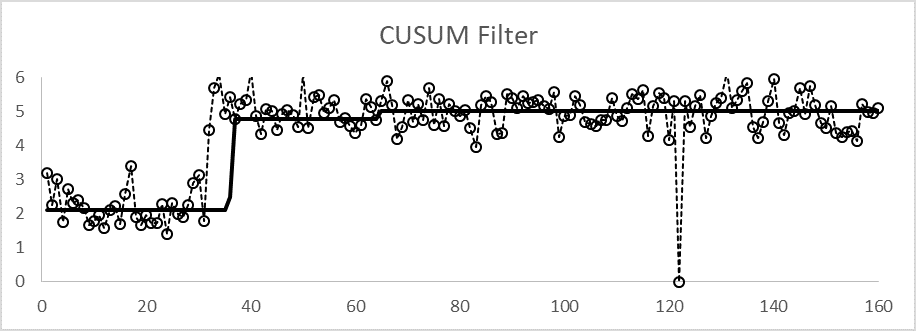
Figure 3 illustrates the CUSUM filter on the same data. Note that the filtered signal does not change during the initial steady state period and quickly jumps when there is a real change. It took about five samples to be statistically confident in the change from 2 to 5. In this set of data, the filter did not jump quite far enough, but made a correction after samples in the 40 to 60 period provided adequate confidence. Also note that the outlier at sample 120 was rejected.

---

The statistically based filters are scale independent; they adapt to the noise amplitude. One author often applies the CUSUM filter to the output of a controller to temper control action, rather than to mask the input CV activity. However, adding a deadband or rate limiting to the output is also effective in tempering the controller, although such action is not self-adaptive to changes in noise amplitude. Statistical filters are also useful to temper process coefficient adjustment.

A statistically based filter moves rapidly when a change is confidently detected and holds a constant value in between. When the process noise amplitude changes, the responsiveness automatically changes. However, the code for this CUSUM filter is about 10 lines and requires that the noise be relatively compliant with the basis of independent sample-to-sample fluctuations. The user interpretation of the statistical trigger will be unfamiliar to many.

Kalman: The Kalman filter is a statistical filter that is significantly more complicated than other filters summarized in this article. It compares data to a model, then reports the value that has greater statistical confidence. Although common in the electronics and aerospace industries, where linear models are appropriate, and fast computers are justified, it is not common in the CPI.

Outlier removal filters

Here the concept is that the signal is steady, but an occasional event happens to provide a one-time (or brief), wholly uncharacteristic value. This is often called an outlier, phantom, or a spurious event. The filter purpose is not to average, but to ignore that outlier, which might be related to occasional dropped data or an electrically induced spike. Electrical sources include voltage or current surges from a nearby lightning strike, radio communications (RFI), nearby motors starting up, or electric floor scrubbers. Loose or corroding wiring connections, sensors that receive mechanical shock, or dropped data packets in an overloaded communication system can also cause short-lived or one-sample outliers.

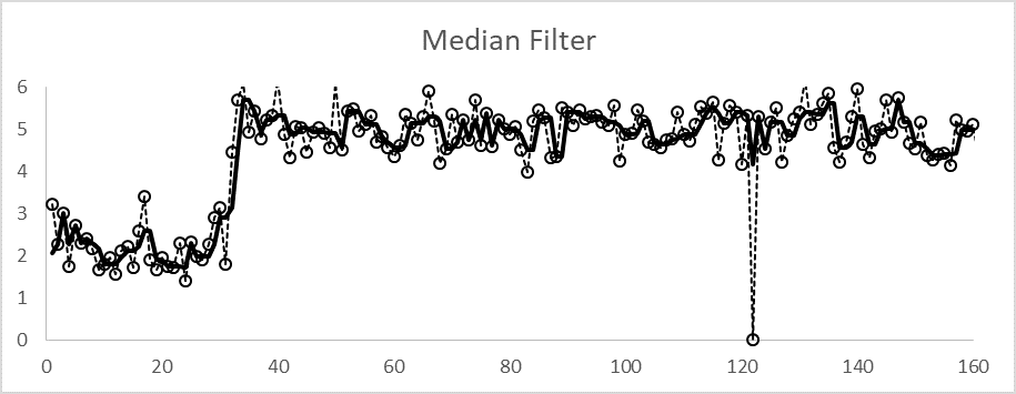
Median filter:The median filter reports the middle of the most recent values—not the middle in chronological order, but the middle in value. For instance, if the three most recent values are 5, 6, and 3, the middle value 5 is reported. Often, redundant sensors are used in which the middle of three measurements is taken as the process value, in a procedure termed voting. However, voting is a special case of parallel measurements at the same time. In a median filter, the middle-of-three is from a sequence of data. A median filter could be based on three, five, seven, or so sequential data. If you suspect that two outliers could happen sequentially, because of some common cause, then a median of 5 will reject them. The median filter does temper noise a bit, but the application intent should be to remove outliers.

Figure 4 illustrates the median filter (middle of 3) applied to the same set of data. Note:

• When the signal makes a step change at the 30th sampling, the filter has a delay of about half the number of data.
• The outlier at sample 120 is wholly ignored.
• Throughout, the vagaries of the signal substantially mimic the measurement.

---

 

Note: The median filter removes outliers and rapidly tracks real changes. However, the user must choose an N that is large enough to exclude persistent outliers. Masking outliers can misrepresent important features, and noise is not removed.

Data reconciliation: Here the concept is that a sensor, or several sensors, acquire a systematic bias, and the reported measurements are not only subject to random noise but also systematic error. Good and frequent calibration could eliminate this problem, but often continual instrument recalibration is not convenient. In data reconciliation, the objective is to use simple process models to back out the values of the systematic errors from the data. It is a powerful technique, but requires valid models, redundant process measurements, and online computing that is an order above the other algorithms discussed here.

Heuristic methods: These are user defined, as appropriate, and could be based on any number of data consistency or validation checks that a human observer might use to judge veracity. For instance, if a sudden change in one measurement correlates to a simultaneous or prior change in another, then the one-time effect may be interpreted as real, not an outlier. The logic is usually implemented as “if-then-else” rules that pass through valid data and perhaps flag what appear to be outliers. Flagged data could then be “thrown out” or ignored by process control applications, but still be retained for historian recording purposes.

The creation and management of large sets of if-then rules for data validation as well as other applications (e.g., real-time process diagnostics, intelligent alarming) is a strength of real-time expert systems. However, most commercial automation systems can easily handle the use of small to medium if-then-else rule sets.

Although mathematical equations are the basis of conventional filters, human logic statements can be powerful additional ways to “clean up” data. As a caution, it can be easy to generate conflicting heuristics. While expert systems can help, their use represents an additional paradigm for users to learn and support .

Other filters

Aliasing is when a stray, high-frequency signal confounds a sampled data signal. Sources include harmonics from rotating electrical motors, power transformers, and radio transmission. An anti-aliasing filter rejects the confounding signal. In many industrial platforms, an anti-aliasing filter is a simple first-order filter with a time constant set slightly faster than the base scan rate for the I/O system. This will mostly eliminate the effects of any signals with periods faster than what the controller can respond to and prevent them from being “felt” as a slower, longer period disturbance. High-quality input cards with appropriate anti-aliasing filters will eliminate radio effects for most common process signals.

There are many filters in the loop that may attenuate noise from various sources. For example, a thermowell acts as a filter to temper temperature fluctuations in the fluid when vapor and liquid are in transport. Lags in sensors, such as ion transport across the pH membrane, temper concentration fluctuations. Averaging in sample accumulation before analysis tempers fluctuation. The process engineer may have adjusted a derivative filter, tuned a valve positioner, or added deadband on a controller output or actuator. The process engineer may have selected signal damping effects on an orifice dP transducer. Additionally, many sensors in industry today come with their own microprocessor providing selected features, with some including embedded data filtering for which some adjustment (i.e., tuning constant) is available to customers.

While we acknowledge such diverse applications, this article focuses on techniques that are typically programmed or configured into process control or data historian computers for which users have significant discretion for their use and configuration.

Perspectives

• Filtering can be used to either temper noise or eliminate outliers. Use the right tool for the disparate applications.
• If the signal is noiseless (and void of outliers), then there is no need to consider filtering.
• Some applications (driven by regulatory considerations) may also indicate no use of filtering.
• If the noise level changes, then the user needs to adjust the filter factor to maintain the desired balance of noise attenuation to lag.
• Statistical filters automatically adapt to changes in noise amplitude.
• Filtering adds a lag or delay, which could impair control action, or require alternate controller tuning.
• Diverse filtering methods can be used in combination, such as a median filter to reject outliers, then a FoF to reduce noise.
• Filter effects and options are on nearly every device. Recognize where these might be.

• Facebook
• Twitter
• Linked In