

- By James Beall
- Automation Basics
Summary

By James Beall

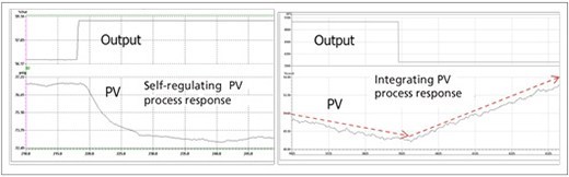
Figure 1. Response of the PV to a step change of the controller output for a self-regulating and an integrating process
Self-regulating responses are very common in the process industry. Many flows, liquid pressures, temperatures, and composition processes are self-regulating. In the March/April issue of InTech, I presented techniques for tuning a PID controller used on an integrating process. In this article, I will present a method to tune PID controllers on self-regulating processes.
Challenges
Regardless of the tuning of the PID controller, the control performance is limited by the performance of the instrumentation and final control element. Before tuning a controller, it is helpful to have an understanding of the process and to verify the performance of the instrumentation and final control element, usually a control valve. The control valve should have a small deadband and resolution - another topic of discussion! It should have an appropriate and consistent flow gain. It should have a response time that is appropriate for the process performance requirements. ANSI/ISA-75.25 and the EnTech Control Valve Dynamic Specification V3.0 are excellent sources of information on this topic. Also, the control scheme should be reviewed to make sure it is an appropriate, linear, control scheme for the application. Finally, the interaction of the control loop to be tuned with other control loops should be reviewed and understood. The desired aggressiveness of the loop tuning should be based on the interaction of the control loop with other loops and the consequences of movement of the controller output.
Tuning for a self-regulating process
A tuning methodology called lambda tuning addresses these challenges. The lambda tuning method allows the user to choose the closed loop response time, called lambda, and calculate the corresponding tuning. The lambda closed loop response time is chosen to achieve the desired process goals and stability criteria. This could result in choosing a small lambda for good load regulation, a large lambda to minimize changes in the controller output and manipulated variable by allowing the PV to deviate from the set point, or somewhere in between these two extremes. More importantly, the lambda of the loop can be used to coordinate the responses of many loops to reduce interaction and variability.
Lambda tuning for self-regulating processes can result in a closed loop response that is slower or faster than the open loop response time of the process. Though lambda is defined as the closed loop time constant of the process response to a step change of the controller set point, the load regulation capability is also a function of the lambda of the loop. The response to a step set point change and a step load change for a self-regulating process response with lambda tuning is shown in figure 2.
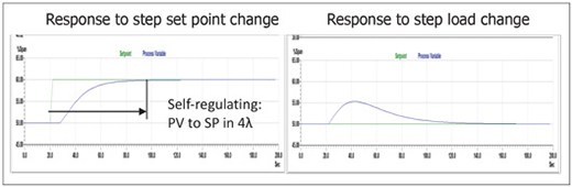
Figure 2. Response of lambda tuning for a self-regulating process for a step set point and a step load step change
Self-regulating process responses typically include dead time and can usually be approximated by a first-order or second-order response. This article describes the lambda tuning procedure when the process response can be approximated by a first-order-plus-dead-time response. The lambda tuning for a second-order-plus-dead-time response will be covered in future articles.
Procedure
The lambda tuning method for self-regulating processes involves three steps:
- Identify the process dynamics.
- Choose the desired closed loop speed of response, lambda.
- Calculate the required PID tuning constants.
Figure 3 shows the dynamic parameters of a self-regulating, first-order-plus-dead-time process, which include dead time (Td), in units of time; time constant (tau), in units of time; and the process gain (Kp, in units of percent controller PV span/percent controller output span. Typically several step tests are performed; the results are reviewed for consistency; and the average process dynamics are calculated and used for the tuning parameter calculations. If the controller output goes directly to a control valve, any significant deadband in the valve will reduce process gain if the output step was a reversal in direction. If the controller output cascades to the set point of a slave loop, the slave loop should be tuned first.
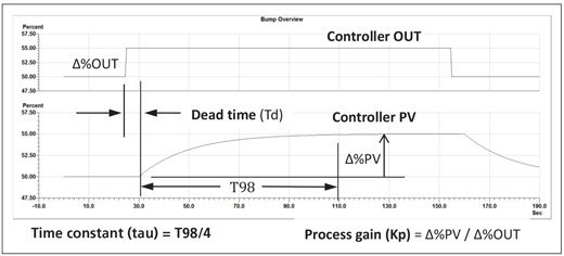
Figure 3. Open loop process dynamics of a first-order, self-regulating process include dead time, the time constant, and process gain. T98 is the time required for the process to reach 98 percent of its final value.
The next step is to choose the lambda to achieve the desired process control goal for the loop the allowable stability margin and the expected changes in process dynamics. A shorter lambda produces more aggressive tuning and less stability margin. A longer lambda produces less aggressive tuning and more stability margin. It is not uncommon for the process dynamics, particularly the process gain, to vary by a factor of 0.5 to 2. If testing during different conditions reveals that the process dynamics change significantly, then an additional margin of stability is required. Or, the process response can be linearized or adaptive tuning can be used.
If the potential change in process dynamics is unknown, starting with lambda equal to three times the larger of the dead time or time constant will provide stability even if the dead time doubles and the process gain doubles. If it is desirable to coordinate the response of loops to avoid significant interaction, the lambda of the interacting loops can be chosen to differ by a factor of three or more. For cascade loops, the lambda can be chosen to ensure the slave loop of the cascade pair has a lambda 1/5 or less of the master control loop.
The lowest recommended lambda for a first-order-plus-dead-time self-regulating process is equal to the dead time, although this provides a very low gain and phase margin. Thus, a smaller increase in the dead time or process gain can cause instability of the loop.
From a stability standpoint, there is no upper limit on the lambda. If the lambda is not chosen based on a coordinated response, a good starting point for stability is:
Equation 1.
Lambda = 3 * (larger of dead time or time constant)The tuning performance can be monitored for a time period and adjusted to be a shorter or longer lambda as needed.
The final step is to calculate the tuning parameters from the process dynamics. Care should be taken to use consistent units of time for the dead time and the lambda. For a first-order-plus-dead-time process response (no significant lag or lead), the controller gain and reset times are calculated with the following equations. The derivative time is set to 0. These equations are valid for the standard (sometimes called ideal, noninteractive) and series (sometimes called classical, interactive) forms of the PID implementation. Note that only the controller gain changes as lambda (λ) changes. The integral time remains equal to the time constant regardless of the lambda chosen.
| Equation 2. | |
| Integral time = | time constant (tau) |
| Equation 3. | |
| Controller gain = | (Integral time) |
| |Kp| (λ+Td) | |
Example
Consider the steam pressure controller shown in figure 4. The pressure controller, PIC-101, manipulates a properly sized control valve that has a high-performance digital positioner.
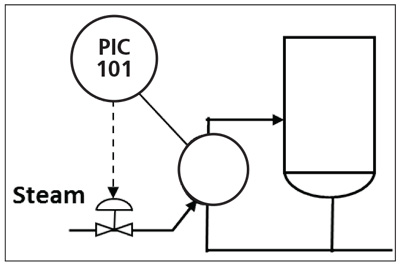
Figure 4. Process and control diagram for a reboiler shell steam pressure control
Figure 5 shows a step test of the pressure controller to identify the process dynamics. The process gain is %PV/%OUT; the dead time is 5 seconds; and the time constant is 20 seconds.
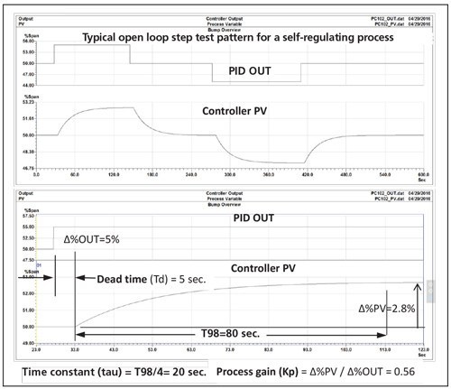
Figure 5. Open loop step test and analysis of one step response
Because there are no loop response coordination requirements, the initial lambda is chosen to be 3 * (larger of dead time or time constant) = 3*20 seconds = 60 seconds.
Now, the tuning can be calculated with the lambda tuning rules.
| Integral time = | Time constant (tau) = 20 seconds | |
| Controller gain = | (Integral time) | |
| |Kp| (λ+Td) | ||
| = | 20 seconds/((0.56)*(60 sec+5 sec)) = 0.55 | |
| Derivative time = | 0 seconds | |
In preparation for being able to make the tuning more aggressive if the control loop is consistent over the required operating range, the tuning can be calculated for shorter values of lambda. The following table shows the tuning for different values of lambda. Note that the integral time remains the same for all choices of lambda.
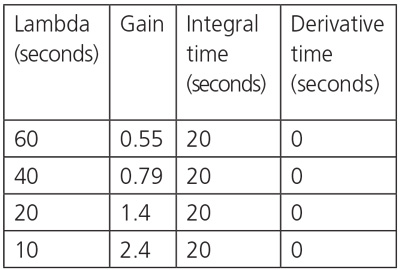
Figure 6 shows the response to a step set point and a step load change for each of the lambda values in the table. Note that the tuning is stable for much shorter lambda values than the starting point of 3 * (larger of dead time or time constant). However, this is with perfectly constant process dynamics in a simulator. Additional tests on a real process, at different operating conditions will help determine how consistent the process dynamics are.
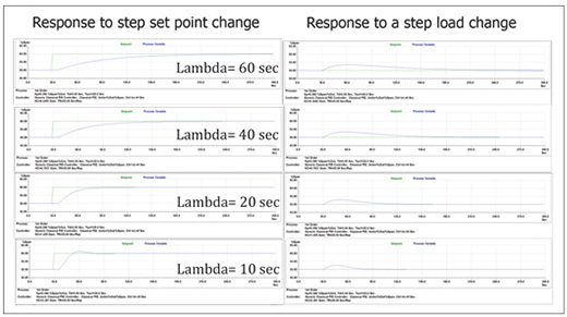
Figure 6. Response of self-regulating process for a step set point and step load change with different lambda values
Meeting process goals
Most published PID controller tuning methods are designed for optimum load regulation, not necessarily optimum process performance. The lambda tuning method provides the ability to tune the PID controller to achieve process performance goals, whether they are maximum load regulation or a coordinated response to other loops. Note that the lambda tuning method for integrating processes can also be used for a lag dominant, self-regulating process to achieve excellent load regulation. This technique and tuning for more complex dynamics will be covered in a future article in this series.
Reader Feedback
We want to hear from you! Please send us your comments and questions about this topic to InTechmagazine@isa.org.