State-Based Control Solutions for Complex Systems

• By Robert Rice, Ziair DeLeon
• Continuous & Batch Processing
• Oil & Gas

Summary

One producer tamed a difficult level control task, improving test separator performance.

Anyone who has ever worked in the Canadian Athabasca oil sands production fields knows that the term “tar sands” is far more accurate. While oil is ultimately produced, it begins as bitumen, the heavy crude that is almost solid. Extracting it from wells demands steam-assisted gravity drainage (SAGD) techniques where each well is a combination of two drilled holes (Figure 1). One well injects steam to heat and soften the bitumen, separating it from the sand, and the other producer well pumps it out. What results is a mix of bitumen, natural gas, solids, and water. While this process is energy-intensive and expensive, numerous companies are using it and producing a total of about 1.3 million barrels per day across the region.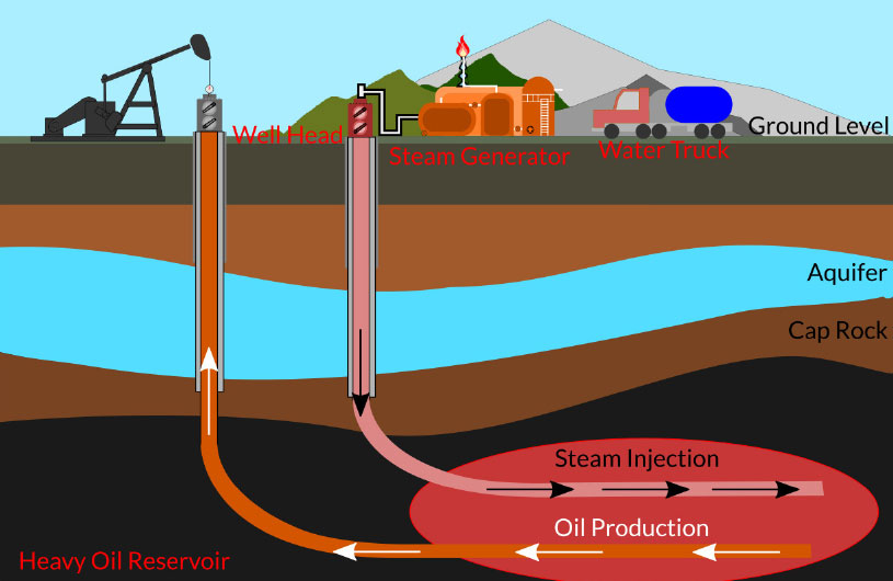

Most companies engaged in this effort operate large production sites with multiple pads consisting of 10 to 20 well pairs sharing common infrastructure. Since the output of any well is a mix of products and contaminants, multiple steps are required to recover and concentrate the actual crude oil while removing lighter hydrocarbons and contaminants. The first stage of separation combines all the wells into a single stream and removes gaseous compounds so the liquids can be treated subsequently. Later, water and oil are separated. Recovered water is usually treated and reused.

Real-world production facilities rarely present ideal scenarios. They are invariably driven by numerous conditions and interactions, providing impediments as well as opportunities.

This first separation stage provides the earliest opportunity to evaluate the output from a given well so operators can judge the actual production volume with its proportion of bitumen against water, entrained solids, and contaminants, including undesirable sulfur compounds. Well output is anything but consistent since bitumen deposits are non-uniform even over short distances. Consequently, different wells, even at the same site or pad, can have much different output. Characteristics of a given well can also change over time as different portions of material liquify and are extracted.

To evaluate individual wells, a much smaller test separator is often used (Figure 2), in conjunction with piping and valve manifolds, so that any one of the wells can be directed by itself to the test separator rather than the collective unit. This allows operators to examine and characterize each individual well, determining the quality and quantity of its output. For a typical operation, the control system might configure each well to the test separator for 12 hours, stepping through each well in sequence.

Controlling level

The test separator is not a grab-sample system. For the 12 hours it is connected to a specific well, production must continue normally, so the flow is continuous. To do its job, a specified level must be maintained in the separator. When working properly, the test separator performs the same task as the main separator, but at a smaller scale and only for one well at a time.

Assuming an example production site with 12 wells, each well would get its time on the test separator every six days. The test separator drum is very small compared to the main separator, perhaps less than 100 gallons, and it is critical to maintain a consistent level in the drum for it to function properly. Due to difficulties instrumenting this type of flow stream, there is no flow meter on the separator inlet, so the task becomes a basic level loop. Conventional wisdom says creating an effective level loop is difficult under the best circumstances, but this situation introduces additional complications.

For example, when switching wells, there is no way to know what the incoming flow will be. The wells do not produce consistently when compared to each other, nor does any single well produce consistently all the time. When well No. 1 is tested on a given day the level loop may be stable, but the quantity and character of its output will likely be different when it is tested again almost a week later. So how can operators hope to maintain control of the test separator level loop in the face of such chaotic conditions?

Applying loop analysis tools

For the last 20 years or so, control loop performance monitoring (CLPM) tools have been available to help oil refiners, chemical plants, and other process manufacturers improve the interaction of hundreds and even thousands of related PID loops controlling a process. By analyzing operational data, these traditional CLPM solutions identify undesirable PID performance characteristics, facilitate the isolation of root-causes, and even recommend issue-specific corrective actions.

These tools have proven very effective at providing a generalized assessment of controller performance based on in-use data. Unfortunately, they are often limited to a single basic operating condition, generally when the plant is stable and running “normally,” whatever that means for the plant or unit. For the case of test separator level control, the picture is much different than a typical process unit. The biggest difference is the scope of the problem. Instead of hundreds of loops, the operators are concerned with a single isolated level loop for the test separator where tuning parameters need to change every 12 hours and be associated with a unique source. Conventional CLPM tools simply do not apply.

Adding state-based analytics

More sophisticated CLPM tools that have emerged in recent years now incorporate state-based analytics capable of distinguishing a process’s many and unique operating states. They develop and apply multiple operating profiles, or operational states, that can be dynamically applied to a control loop’s performance metrics. Depending on the operating situation, state-based analytics allows operations staff to gain a more accurate assessment of loop performance as processes shift between different phases of manufacturing, making users better informed and more capable of improving production performance.

States add context to the source data and are configurable based on any combination of operating phases, products, run-time conditions, or other production-related attributes. Even distinct batch sequences can be addressed in this manner.

For our example well site, a more advanced state-based version of CLPM proved ideal for analyzing a control loop with 12 entirely unique operating conditions.

State attributes are determined by the CLPM solution using process and condition data accessed from a plant’s data historian, so that state-based analytics techniques can be applied for like-to-like conditions throughout an operation. This makes it possible—based on what state the system is in—to proactively detect negative performance trends and enable users to understand and address issues more precisely, such as variable tuning, operational constraints interfering with effective control, and loop interaction problems. For the case of our example well site, this more advanced state-based version of CLPM proved ideal for analyzing a control loop with 12 entirely unique operating conditions.

Applying state-based analytics

In this case, because the control system is used to configure the valve manifold to connect a given well with the test separator, it is straightforward to designate 12 unique states. Of course, more states are possible if there are other uniquely detectable conditions. Figure 3 clarifies how this works. It shows a few days of data from the process, with 12-hour periods for several wells. The set point of the level loop during production would normally remain constant for effective separation, although this figure happens to depict setpoint changes that were initiated to characterize the system and generate models used to build the adaptive PID settings. Clearly, the amount of control effort necessary to maintain the set point changes drastically. This may be related to tuning, but also likely instability of well output across the test period.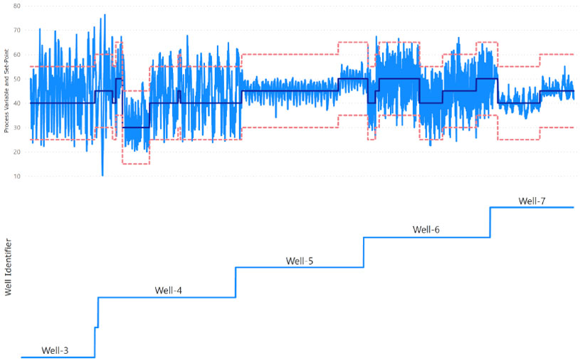

Analytical results

Prior to Control Station’s involvement at the site, there was little differentiation between the level control success of each individual well. When assessing overall performance, the traditional CLPM approach operated on the aggregated data from many varying states. The assessment included computations related to PID tuning, mechanical performance, and process interaction. But without the ability to distinguish the performance of individual well pairs, the result was a set of values not specifically helpful for any of the states.

The key performance indicator (KPI) in this case was an average absolute error (AAE) value. It is a common assessment of controller performance and quantifies the difference between the set point and measured process variable for a given PID loop. Naturally for a dynamic process such as this application, some degree of variability should be expected and tolerated. Still, any notable increase in AAE generally corresponds with a change that production staff should at least note if not investigate and address.

When data from the test separator process was examined using traditional CLPM capabilities, the AAE (as an overall average calculated across available well pairs) was 4.8. For this operator, the average value was not considered excessive, and seemed to suggest that the controller was performing reasonably well when having to regulate liquid level across so many different well pairs. However, a decent average can hide some truly bad actors.

Once data on individual wells was available using the state-based analysis, it was clear that there were excellent wells with values below 5.0, along with five underperformers well above that value (Figure 4). Determining why those bad actors were so far above the average and solving the underlying problems went a long way to optimizing the overall performance of the test separator, and the site as a whole.

Once each well could be treated as its own state, it was possible to implement a PID strategy with gain scheduling to bring the loop under tighter control (Figure 5) for all states, reducing all AAE values below 5.0 and resulting in a much better average value of 1.7. Analysis revealed that there was a reasonably strong correlation between the average flow rate and the recommended controller gain, allowing an improved control strategy to be developed. This stabilizes production during each well’s time on the test separator and presents a clearer picture of the output. Analytical tools allow users to “expand” the data to recognize any one state, or they can “collapse” the data to consider averages of one or more states, depending on the need.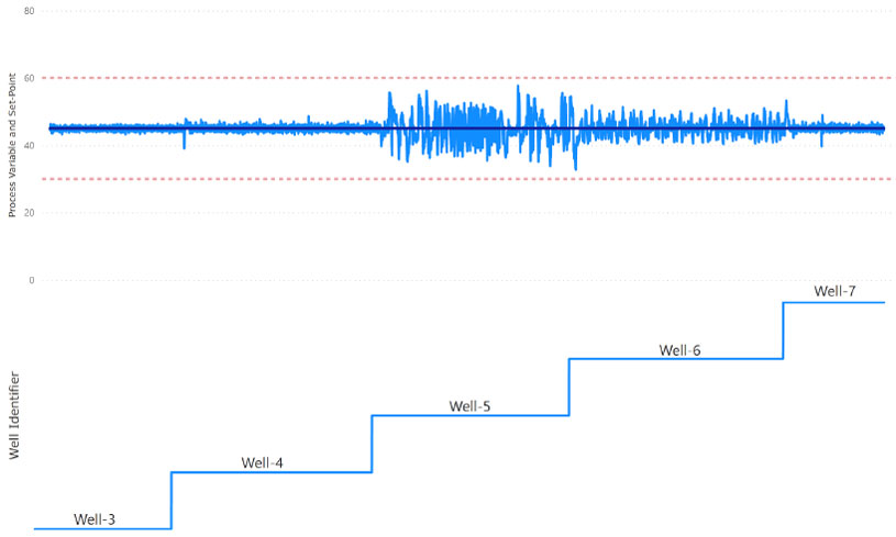

By analyzing operational data, traditional CLPM solutions identify undesirable PID performance characteristics, facilitate the isolation of root-causes, and even recommend issue-specific corrective actions.

Prior to the tuning effort, the end user experienced issues where the separator would exceed alarm limits and cause a unit to trip, so operators ended up babysitting the units more than seemed reasonable. After analysis and subsequent tuning, the system runs more consistently in automatic so far less operator intervention is required, and there are fewer trips.

While traditional CLPM tools have proven helpful in assessing the performance of basic loop operations, state-based analytics is showing particular value within more complex systems. Real-world manufacturing and production facilities rarely present ideal scenarios. They are invariably driven by numerous conditions and interactions, providing impediments as well as opportunities. The combinations of these attributes can be enormous, and the effect of individual combinations on production can be lost within broader trends.

The addition of state-based analytics now makes it possible for CLPM users to delve deeper, facilitating the detection, analysis, and adjustment of operational conditions that had previously stood in the way of plant-wide process optimization.

• Facebook
• Twitter
• Linked In